- Channels and Cycles -Brian Millard - Chapter 7 - 1999
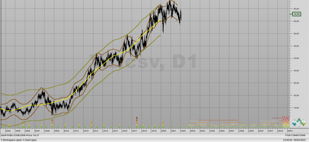
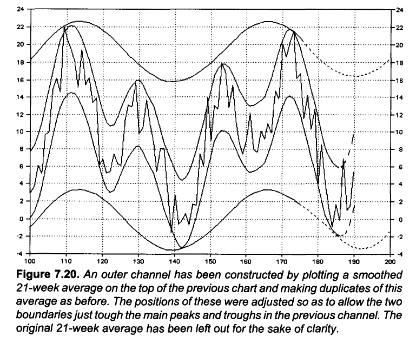
In order to isolate the 52-week cycle we can use a smoothed 21-weekaverage, knowing that this will remove the 21-week cycle and the random data. Now that we know the process we place the channel boundaries as exact duplicates above and below the original position of this average we can leave it out of the plot, Figure 7.20.
This channel is super-imposed on the channel drawn in Figure 7.19. The boundary positions have been adjusted so that the main peaks and troughs in the inner channel just touch the outer boundaries.
The depth of this second channel is just over $18. Since the channel rep-resents the 52—week cycle, this means that the channel contains all fluctuations of wavelength of less than 52 weeks, i.e. wavelengths of 21-weeks or less, and they have a combined magnitude of $18.
Since we have established that the random movement is just over $8 in magnitude, this leaves a difference of $10, which is our estimate of the magnitude of the 21-week cycle. We know the latter in the original data to have been $10, so this estimate is excellent.
Although we could draw a third, outer channel by selecting a smoothed average with a span greater than 52 weeks, it is hardly necessary in this case because the outer channel will be running horizontally.
The upper boundary would be drawn to touch the 2 peaks in the second channel just drawn, while the lower boundary is drawn to touch the troughs in this channel.
The depth of such a channel is the vertical distance from peak to a trough in the second channel. This is approximately $26, and is due to all the cycles and random behavior present.
From the way the test data was created in the first place, this total should include :
- $10 for the magnitude of the 52 week cycle,
- $10 for the magnitude of the 21 week cycle
- and $8 for the magnitude of the random behavior,
i. e. a total of $28 in all.
Thus our estimate of $26 is quite good. By difference between the 2 channel depths, we estimate the magnitude of the 52 week cycle as being $26 - $18 = $8.
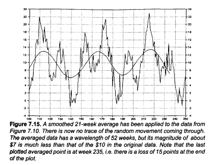
The reason for the estimate of this magnitude being slightly low is be-ause of the overall effect of the application of averages in reducing the magnitude of the cycles which the average lets through.
We saw this effect in Figure 7.15.
In order to isolate the 52-week cycle we can use a smoothed 21-weekaverage, knowing that this will remove the 21-week cycle and the random data. Now that we know the process we place the channel boundaries as exact duplicates above and below the original position of this average we can leave it out of the plot, Figure 7.20.
This channel is super-imposed on the channel drawn in Figure 7.19. The boundary positions have been adjusted so that the main peaks and troughs in the inner channel just touch the outer boundaries.
The depth of this second channel is just over $18. Since the channel rep-resents the 52—week cycle, this means that the channel contains all fluctuations of wavelength of less than 52 weeks, i.e. wavelengths of 21-weeks or less, and they have a combined magnitude of $18.
Since we have established that the random movement is just over $8 in magnitude, this leaves a difference of $10, which is our estimate of the magnitude of the 21-week cycle. We know the latter in the original data to have been $10, so this estimate is excellent.
Although we could draw a third, outer channel by selecting a smoothed average with a span greater than 52 weeks, it is hardly necessary in this case because the outer channel will be running horizontally.
The upper boundary would be drawn to touch the 2 peaks in the second channel just drawn, while the lower boundary is drawn to touch the troughs in this channel.
The depth of such a channel is the vertical distance from peak to a trough in the second channel. This is approximately $26, and is due to all the cycles and random behavior present.
From the way the test data was created in the first place, this total should include :
- $10 for the magnitude of the 52 week cycle,
- $10 for the magnitude of the 21 week cycle
- and $8 for the magnitude of the random behavior,
i. e. a total of $28 in all.
Thus our estimate of $26 is quite good. By difference between the 2 channel depths, we estimate the magnitude of the 52 week cycle as being $26 - $18 = $8.
The reason for the estimate of this magnitude being slightly low is be-ause of the overall effect of the application of averages in reducing the magnitude of the cycles which the average lets through.
We saw this effect in Figure 7.15.
Attached Images
2