Thanks FXEZ for putting up this thread and thanks guys for your valuable contributions. Very interesting stuff here that really helps seperate the wheat from the chaff. :-)
Ignored
Thanks for dropping by Copernicus! Hope you get something out of it!
Although I have zero experience with R (or things like matlab) and relatively modest experience with other languages (mostly mql, c and some web, html..) over the years I've managed to make quite a few experiments regarding algo trading (and trading prob.stats. as a whole). So, I am able to share some of my experiences and insights. I have no intention to post my code here, only my theoretical conclusions and philosophical insights based on my research. If the OP considers the following for off topic - feel free to delete my post! ------------------------------------------------------------------------------------------------...
Ignored
Thanks for your post alphaomega - very comprehensive and among other things stresses cost of trade execution - something that is often overlooked! I hope you will continue to contribute your findings here. I really appreciate it.
Thanks for your post Tardigrade, I'm glad that you're here. You make an excellent point about random number generators and their limitations. Have you used hardware based random number generators? I wonder how easily these hardward RNGs integrate with programming environments like R or Python and how they are in terms of speed vs software algorithms?
The R code then imported the data and cleaned it. It calculated the approximate dollar value for a 1 pip move. The analysis is then based off of this. ** FXEZ (or anyone else) -- do you think this is the best way to do this? The other way is to do the linear regression analysis on raw prices ... but the problem is that some currency pairs are orders magnitude different (think JPY crosses: xxx.xx and EURUSD: x.xxxx). This makes the coefficient very small or very large. I have thought of doing % change from previous bar also ... but want to get the...
Ignored
ezcurrency: It's been a while since I've played with cointegrated baskets. It seemed like the best input to use was converting price moves to dollar moves so you have a common denominator (as you have done). Also being aware of the JPY crosses' 100 multiplier and making the necessary adjustment to get the coefficients on the same scale as the other prices is a must. By using a fixed number for the currency conversion you ensure the need to reoptimize from time to time when values shift, but that's probably necessary regardless. Doing it the continuous way is much messier (lots of code) and you may not get that much more benefit out of it vs what you are doing - the spreads still tend to drift so you have to keep reoptimizing over time.
Quote
Disliked
Now that we have the data frame 'x' of all prices (data massaged and scaled as described above), we normally would do a linear regression of each pair on each other to calculated the coefficients and then calculate the spread. The problem is if we use linear regression of x on y, we get coefficient c. Now if we do a linear regression of y on x, we might not get coefficient 1/c.
Yes that's a good point - Paul Teetor addressed that in a paper that basically came to the same conclusion, and I tend to agree that getting stability in the coefficients is very important. Alternatively you could compute lm(y~x) and lm(x~y) and average them but that seems like a lot of work when we already have princomp, particularly if you are dealing with this problem with more than 2 symbols.
The rest of your approach seems reasonable as well. Requiring the spread to be above its MA before buying seems like a good way to avoid fading trends. The bottom line is of course how it performs going forward. Really nice contributions, ezcurrency!
{quote} One can use correlation coefficient which does not depend on absolute values of tested variables. I am also not sure that prices are normally distributed.
Ignored
Thanks for your comment, vg10. Are you saying compute the cointegration on the correlation coefficient series? If you are using two symbols you only have one correlation series. How would this work in practice?
{quote} Thanks for your post Tardigrade, I'm glad that you're here. You make an excellent point about random number generators and their limitations. Have you used hardware based random number generators? I wonder how easily these hardward RNGs integrate with programming environments like R or Python and how they are in terms of speed vs software algorithms?
Ignored
I'm planing to buy one of those and still doing my research before buying
In the meantime, for quick integration with R, random.org should suffice.
Joined Aug 2010
|
Status: Stare Into the Lights My Pretties!
|779 Posts
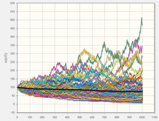
Look at this chart very carefully!
These are 100 equity curves with 1000 trades each.
Attached Image (click to enlarge)
What do you see? Do you notice these exponentially rising trends, which are rising to 100%, 200%, 300%, 400%......
These curves are 5 - 8% of all curves.
They look pretty good!?
What do you think?
-----------------------------------------------------------------
What you don't realize(at first), is the fact that ALL of these curves are generated by system with NEGATIVE(small, but negative) mathematical expectancy per trade!
This means that eventually over time ALL of these curves will go to zero!
However, if you look at all these positive curves ( the "winners") and study each one of them on individual basis, you will find that they all have positive expectancy per trade (based on their history). Despite the fact that they are generated by system with negative expectancy!
What this means is that, LUCK can persist for a very long time! These are 1000 trades each! I can simulate 10 000 trades and you will still find a few "consistent" "winners".....producing positive expectancy per trade.
It's perfectly normal from statistical standpoint.
Now imagine what the situation will be, if you never knew how these curves are generated!
What if I just pick only the best 10 curves out of 1000 simulations (with all their individual statistics), and tell you that these are made by successful professional traders.
Think about this for a moment!
You can also go to the "leader" board section of this site.......just to notice that the list with "leaders" is limited to ONLY 100 traders! (despite the fact that right now there are 11,628 traders with trade explorers linked to FF.
Just some food for thought........
------------------------------------------------------------
The reality is that you can be wildly successful trader for quite some time, without realizing that this spectacular success is generated by system with negative mathematical expectancy. Then eventually when the law of large numbers starts to kick in, and the equity starts to collapse with spectacular speed (reverting to the mean). - you just say - well, the market "changed" and "my system stopped working". Sounds Familiar?
What you don't realize is that your system never worked in the first place, and you are just one lucky poor soul for not knowing the difference!
Now think about the possibilities (statistically).
What percentage of all successful (and famous) traders are just lucky winners? (normal statistical outliers)
I mean, especially for the lower frequency strategies, it may take many years for them to accumulate a few thousand trades.
In the mean time these people are managing OPM. Some of them have hundreds of millions under management! And their investors and everyone in the industry thinks that these traders are superstars!
While many of them truly are superstars, it's possible (based on probability theory) that most are just very very lucky.
What do you think?
I think that the red pill tastes like shit, but at least it gives you some truth!
And only truth will set you free.....Or so they say.
What you don't realize(at first), is the fact that ALL of these curves are generated by system with NEGATIVE(small, but negative) mathematical expectancy per trade! This means that eventually over time ALL of these curves will go to zero! However, if you look at all these positive curves ( the "winners") and study each one of them on individual basis, you will find that they all have positive expectancy per trade (based on their history). Despite the fact that they are generated by system with negative expectancy! What this means is that, LUCK can...
Ignored
The whole life has a negative expectancy.. as in the famous quote -
Quote
Disliked
On a long enough time line, the survival rate for everyone drops to zero
we will all die for sure. Nothing is forever. Success is always just temporary. Very small part of the population become rich and highly successful and that is true for any field. From those who do make it, large percent would not sustain it for a lifetime. And from the very very few that make it and sustain it, we could say that they are just some lucky mfs. Everything is luck. Your genetics, they form the character traits.. they are pure luck. Where and when were you born, who are your parents, your educators, your loved ones.. we think we are so much capable to know and to choose, but the truth is that we are all nothing more than those outliers in a negative end game.. it never ends good. Anything. That does not mean there is no purpose to try and go as far as possible within the given limitations. The harder you work, the luckier you can get.
Joined Jan 2007
|
Status: developing...
|974 Posts
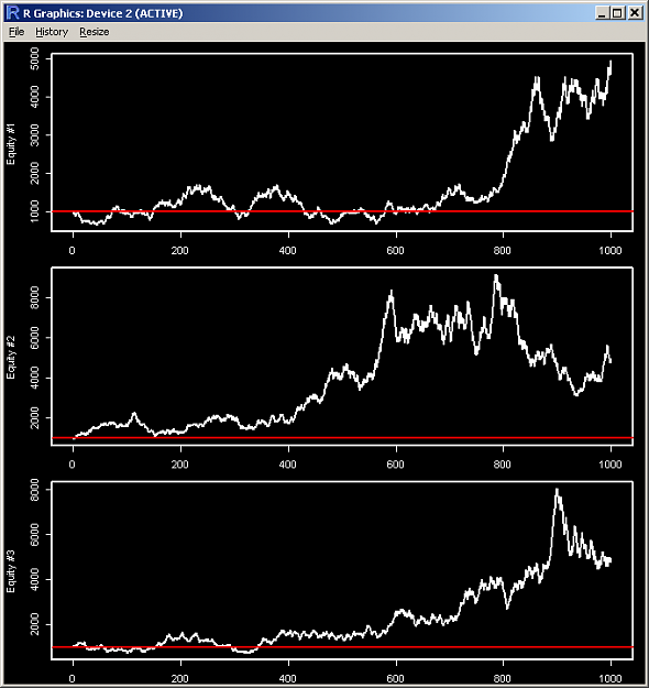
The following three charts represent three different systems. All are profitable. In your opinion, which one is the best of the three? All three systems started with the same amount of money: $1000, and used the exact same money management strategy: percent of equity, and the same leverage: 20x.
Attached Image (click to enlarge)
I computed the Sharpe ratio for the 3 systems and they were as follows:
System #1: 1.61
System #2: 0.72
System #3: 1.11
Now it's becoming quite clear that system #2 is the worst of the three, and system #1 is probably the best. But if you look at another metric: the % of time spent above break-even, system #2 takes the prize, followed by system #3 and then a distant third system #1. What about other metrics?
All three systems ended up with the same ending account balance. Does that change your view of which system was best? What about if I told you that all three systems had exactly a 53% win rate and the exact same reward:risk ratio? What's going on here?
The only difference between the three equity curves is in the sequence of the wins and losses, not in the count of the wins and losses. All systems had 1000 trades with 53% wins and leveraged their current equity by 20 times at each step. But there are 3 different unique win/loss paths followed by the three systems, and all three paths lead to the exact same end point.
So what can I surmise from this? The previous post by alphaomega refers to luck, similar to the tone struck in "Fooled by Randomness" by Taleb. But what about skill? It seems that a great deal of the particular path taken constitutes luck with all its variation, but the fixed end point and expectancy constitutes skill. All three systems have the exact same expectancy, so by this measure all three are equally skilled. But the curves look quite different to the eye and to the Sharpe ratio, even though all three curves arrive at the same terminal balance.
I write this as one who has spent a lot of time analyzing the path of equity curves in search of an advantage. Maybe it has been a hopeless endeavor? These tests were done with simulated data, which, though useful is not the same as real market data. But is that distinction important? I'm starting to wonder...
I also can say that given a fixed number of trades and a fixed win percent and reward:risk ratio, the outcome of a system using percent of equity money management is not path dependent. Or in other words the equity will arrive at the exact same spot even if you randomly change the path of wins/losses. That's an interesting property.
|
Commercial Member
|
Joined Apr 2013
|4,366 Posts
Great stuff Guys. The conclusions drawn in posts 27 and 29 are something to ponder. Most interesting were the conclusions drawn by the importance of key variables by FXEZ on a hypothetical simulation where there was a fixed number of trades, fixed win % and fixed reward to risk ratio, the bolded items being the fundamental constituents of expectancy.
What is clear from FXEZ's analysis however is that markets do not exhibit this constant feature. As a result both the path of the equity curve and the final outcome becomes a variable feast and highly affected by where and when non-random price action is located within the data series.
I have drawn similar conclusions regarding the degree of luck that is present in any equity curve. Alpha appears to be a very small bias in an otherwise random outcome that over the Law of Large Numbers results in positive expectancy, but it is impossible to predict when the non-random features of price action unfold. You need to be very careful in your assessment of the performance metrics of your system in discerning between actual performance results and results attributed to simple chance.
As FXEZ has clearly demonstrated, there is considerable variation in the profile of the equity curve that can simply be attributed to the particular sequence of trades in the return series.
Given this feature, it is useful when assessing the performance metrics of any single trading system to plot where the historic equity curve of a return series fits in a Monte Carlo sequence (where the trade sequence is re-ordered).
Simply relying on performance metrics associated with any historic equity curve is a dangerous exercise unless you consider the result of your backtest in the context of the entire population of possible trade sequences.
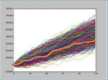
Example 1
Attached Image
For example refer to the chart above (Example 1). The graph displays the historic equity curve (in orange) of a system offering a slight positive expectancy. Simply making conclusions on the historic equity curve alone in assessing your performance metrics can lead you into a serious trap. The orange equity curve has all the characteristics of a system with a high positive expectancy, a low drawdown, high annual sharpe and a good return result......however.....now for the fine print....... how much of this equity curve performance metrics can be attributed to simply the trade sequence?
If we plot the historic return series in the context of the possible different configurations of trade sequence (refer again to the chart above) we find that the historic result is not representative of the average of the series (which would be positioned in the middle of the entire population). The orange equity curve plots at the upper end of the population series indicative of the fact that a large portion of the result can simply be attributed to the favourable nature of this particular trade sequence.
The upper placement of the historic plot in the entire population of series suggests that the equity curve is dominated by simple random good luck with a favourable trade sequence outcome as opposed to a result that typifies the performance metrics of the system. It is likely that a trader using the historic equity curve alone as a guide to future results is going to be disappointed when going live, as they may find, when the trade sample size increases, that the result reverts to the mean of the entire distribution series.
If however I compared the return distribution of Example 1 above to Example 2 below we can more confidently make the following conclusions in regards to overall performance metrics.
Example 2
Attached Image
1. The entire distribution of the MonteCarlo sequence of Example 2 demonstrates that this system possesses a far higher positive expectancy than Example 1. All possible trade sequence outcomes generate a stronger more linear (less volatile) performance result, whereas a large proportion of the population of trade sequences in the prior example were overall losers and correspondingly, the overall volatility profile of individual return series was far more variable. This suggests that for Example 1, the sequence of trades is a far greater dictator of overall performance results than the underlying performance metrics.
2. The standard deviation amongst the total population of possible return series in example 2 is far tighter than the standard deviation of the population of the total possible return series of the prior example, demonstrating that example 2 possesses a far more robust edge that the prior example for the given set of market conditions in this sample. Furthermore the equity curve outcome is dominated by the performance metrics ofthe system as opposed to the simply sequencing of trades.
3. The plot of the historic equity curve fits snugly around the average of the entire population of return series suggesting that the historic result is far more representative of the system performance metrics over the time series concerned, and can therefore be used as a far better guide of future expected returns, provided of course that future conditions are representative of the time series in the sample.
So the moral of the story is that you should never assume that the historic equity curve of your trading system is a suitable proxy for the future unless you closely consider the impact that the sequence of trade results may have in biasing historic performance results.
Can the MM strategy be found that is the inverse of the % of equity sizing such that instead of a negative drag we get a positive boost to the account?
Ignored
Whatever the money you bet it always represents some percentage of your equity. Let's be this fraction x, x∈[0, 1].
With a RR=1 the account either grows by a factor 1+x or shrinks by a factor 1-x. If x is kept for each trade, you get the fixed fractional money management (POE).
In a win-loss (or loss-win) sequence the account grows by (1+x)(1-x). You search x such that this is greater than or equal to one (boost or at least no drag).
Inserted Code
  (1+x)(1-x) >= 1
  1-x^2 >= 1
  -x^2 >= 0
Obviously no boost is going to happen since x^2 is non negative. The optimal x is no trading (0%) to get no negative drag!
Therefore the bet size shall change from one trade to the other. But since your (non-)edge doesn't change is it sensible?
Here I distinguish the win-loss and the loss-win cases because after the first trade we can decide to change the risk.
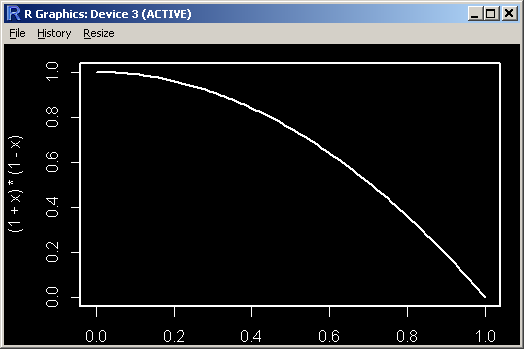
You can plot the functions x and 1 - 1/(1+x) to convince yourself that y is always less than x. After a winner you need to preserve the gain.
For the second case:
Inserted Code
(1-x)(1+z) >= 1
1+z >= 1/(1-x)
z >= 1/(1-x) - 1
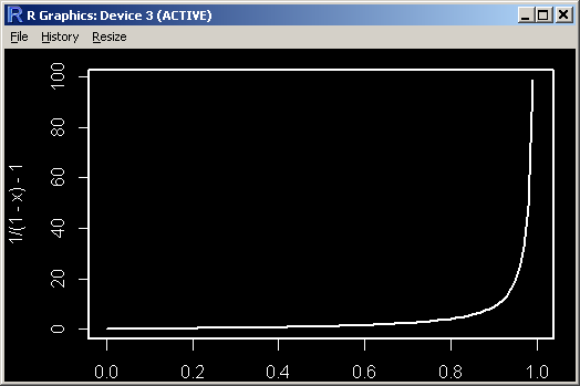
Again you can plot 1/(1-x) - 1 to convince yourself it is above x. You have to increase after a loser to recoup the loss.
So the answer is YES... if you dare entering the land of Lord Martin Gale....
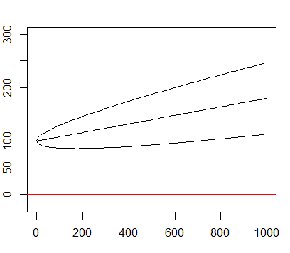
Bernoulli trials are certainly not perfect representatives of market trading activity but they are analytically tractable. We can plot the envelope of all the possible random "equities" within 3 standards deviations simply knowing the winrate and the RR.
Attached Image
The standard deviation of this envelope grows as the square root of the numbers of "trades". The expected "equity" grows linearly.
Good news at some point the mean overcomes the variance: there is a point of maximal DD risk (blue) after which the worst case scenario is stricly increasing.
This implies that at some point (green) the worst case scenario (within 3σ) is above the starting equity and growing.
Bad news: with the values I chose (54%, RR=1) you need 178 trades to pass the max DD point and 699 trades to be safe. That's quite a lot.
In order to reach this point you need a high frequency of trading. Read alphaomega's post again: high frequency trading = huge cost.
You have to be really sure of your edge. I mean statistically not by fooling yourself.
Inserted Code
# Setup the graphics
if (dev.cur() == 1) x11()
par(mar=c(3,2,2,1))
b <- 100   # starting balance
p <- 0.54  # probability of winning
R <- 1     # RRR

E <- p*(R+1)-1       # Expectancy
v <- p*(1-p)*(R^2+1) # Variance
low <- ((3*v) / (2*E))^2 / v # lowest point (3 standard deviations confidence)
pos <- (9*v)/E^2             # (3 standard deviations confidence)
curve((b+E*x), from=0, to=1000, col='black', ylim=c(-20, 300))
curve((b+E*x+3*sqrt(v*x)), from=0, to=1000, col='black', add=T)
curve((b+E*x-3*sqrt(v*x)), from=0, to=1000, col='black', add=T)
abline(h=b, col='darkgreen')
abline(h=0, col='red')
abline(v=low, col='blue')
abline(v=pos, col='darkgreen')
Joined Aug 2010
|
Status: Stare Into the Lights My Pretties!
|779 Posts
Regarding the % risk per trade, based on my research, the optimal solution (especially for discretionary trading) is this:
1. First given that you know what can be expected from your strategy(roughly), you have to estimate the average expected drawdown based on fixed** risk per trade. Lets call this measure "D" (you can think of "D" as one standard deviation of your expected risk)
** By fixed risk I mean for example you can chose to risk 10 currency units per 1000 account units.
2. Second, you keep trading with the same fixed risk, and you only increase the risk (the trade size) when the account balance (or the equity) is above the starting balance for each period + D * x
the parameter "x" can be any number ( 0,5 1, 2, 3) and this will determine how conservative you want to play. (bigger "x" = more conservative).
The idea is to eliminate the variability, on a trade by trade basis and to only increase( or to decrease) trade size by steps, based on large samples of trades.
To put it simple, If you are profitable after N trades(you can also add time component) - then you increase trade size. The main benefit from this is that it helps your recovery rate during drawdown. (if you lose 10%, you no longer have to make 11.1% to get back to BE) Well, technically you do have to make 11,1% to BE, but the average time needed to recover is faster then if you use %risk per trade.
For the downside, if the balance is down by D*x then you reduce the unit risk to the previous level.
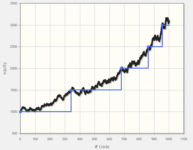
The chart for the trade size will look like staircase.
Here is one example where the main conditions is that we increase the trade size for every 500 units of profit. The black line is the equity, the blue is trade size.
Attached Image (click to enlarge)
The main downside with this approach is that if your system is prone to deep drawdowns, you will have to use larger "x" or smaller unit risk per trade in order to avoid total account loss. And this may reduce the long term gains. (it reduces the speed of compounding)
---------------------------------------------
While mathematically this approach is not the optimal solution, and theoretically using % risk per trade may seem like a better deal, in the real world it's not.
I have drawn similar conclusions regarding the degree of luck that is present in any equity curve. Alpha appears to be a very small bias in an otherwise random outcome that over the Law of Large Numbers results in positive expectancy, but it is impossible to predict when the non-random features of price action unfold. You need to be very careful in your assessment of the performance metrics of your system in discerning between actual performance results and results attributed to simple chance. As FXEZ has clearly demonstrated, there is considerable...
Ignored
Wow, I'm humbled by the great contributions. Nice work guys!
Quote
Disliked
Given this feature, it is useful when assessing the performance metrics of any single trading system to plot where the historic equity curve of a return series fits in a Monte Carlo sequence (where the trade sequence is re-ordered).
It sounds like you're using sampling with replacement of the original system's trade outcomes as in a bootstrapping procedure?
Quote
Disliked
Simply making conclusions on the historic equity curve alone in assessing your performance metrics can lead you into a serious trap. The orange equity curve has all the characteristics of a system with a high positive expectancy, a low drawdown, high annual sharpe and a good return result......however.....now for the fine print....... how much of this equity curve performance metrics can be attributed to simply the trade sequence?
Quote
Disliked
The orange equity curve plots at the upper end of the population series indicative of the fact that a large portion of the result can simply be attributed to the favourable nature of this particular trade sequence. The upper placement of the historic plot in the entire population of series suggests that the equity curve is dominated by simple random good luck with a favourable trade sequence outcome as opposed to a result that typifies the performance metrics of the system.
Can you talk a bit about the procedure you're using to sample the additional curves or create the confidence interval? If you are sampling with replacement I think it is basically saying that you're assuming the population is your total series of trade outcomes (profit/loss) for the system trade by trade. When you randomly sample with replacement from that population of trade outcomes you create new trade series that can have different paths and different expectancies because one curve may oversample winning trades in a series while another may oversample losing trades in a series.
Quote
Disliked
So the moral of the story is that you should never assume that the historic equity curve of your trading system is a suitable proxy for the future unless you closely consider the impact that the sequence of trade results may have in biasing historic performance results.
So the going forward the implication seems to be that even though your long-term expectancy is X, in the short term you may end up with one of the poorer performers rather than the great long-term performer even though the population contains all the trades in the orange curve. In the short term you may get much better / worse than your historic results. Am I in the ballpark?
{quote} You search x such that this is greater than or equal to one (boost or at least no drag). (1+x)(1-x) >= 1
Ignored
Very impressive, PipMeUp! I had a feeling your math skills would come into play in deriving a solution.
A question about your starting formula: It looks like the (1+x) is simply a representation of percent gain and (1-x) would be a percent loss from a starting account of 100%? By multiplying them together (1+x)(1-x) it appears to be the compound interest formula taught in many finance courses. So on the right side of the formula, the >= 1: the 1 represents 100% of starting account?
Quote
Disliked
1-x^2 >= 1 -x^2 >= 0 Obviously no boost is going to happen since x^2 is non negative.
Yes I even tried substituting in the imaginary number i for x and still no joy. By the way, how does one trade sqrt(-1) size?
Quote
Disliked
The optimal x is no trading (0%) to get no negative drag!
Yes I see that in this nice R plot - you get 1.0 on the y axis when your bet size is 0 on the x axis.
{quote} Therefore the bet size shall change from one trade to the other. But since your (non-)edge doesn't change is it sensible?
Ignored
Sensible? If I were a blackjack card counter I would only increase bet size when the deck odds had improved, and possibly with some random variation to throw off the pit bosses. In theory this principle should translate to trading if we can measure the odds going forward. How do we count cards in trading?
Quote
Disliked
Here I distinguish the win-loss and the loss-win cases because after the first trade we can decide to change the risk.
y <= 1 - 1/(1+x) You can plot the functions x and 1 - 1/(1+x) to convince yourself that y is always less than x. After a winner you need to preserve the gain.
Yes I see that - value on y axis is always less than value on x axis.
Inserted Code
curve( 1 - 1/(1+x) )
Attached Image
Quote
Disliked
For the second case: (1-x)(1+z) >= 1 1+z >= 1/(1-x) z >= 1/(1-x) - 1 Again you can plot 1/(1-x) - 1 to convince yourself it is above x. You have to increase after a loser to recoup the loss. So the answer is YES... if you dare entering the land of Lord Martin Gale....
Hmm yes I see what you mean about Lord Martin. He gets a bit wild as x approaches 1.0.
Inserted Code
curve(1/(1-x) - 1)
Attached Image
The last 3 numbers in the sequence are: (eek!)
Inserted Code
[99] 49.00000000 99.00000000 Inf
At around index #50, when x is 0.5 or 50% drawdown then numbers are:
Inserted Code
[50] 0.96078431 1.00000000 1.04081633
so it appears when the account is in 50%+ drawdown you are supposed to risk 100%+ of the account? If it is risk and not bet, then that would translate into leverage much larger than 1.0. It would be like a double or nothing bet at this point right? I'm having problems with the scaling.
Also, regarding the Bernoulli trials post, you effectively demonstrated something that I had noticed in my simulations with equity curves. Your conclusions are a bit depressing but really sum up as drawdown is a fact of life and may last a long time even with a good positive edge. Very nice and a lot to think about!
{quote} It sounds like you're using sampling with replacement of the original system's trade outcomes as in a bootstrapping procedure?
Ignored
Yep, (Edit for clarity: we are simply breaking the historic backtest into sample segments and reordering the segments randomly) over a 100 trade backtest for two different systems, each with a supposed positive expectancy. The point of these examples is that it is important to understand the distribution that your backtest comes from when all other variables are set constant aside from trade segment sequence.
Edit for clarity: The reason I prefer a segment sample approach is to capture some of the autocorrelation that is typically found in clusters in market data. A simple reordering of trades does not produce this effect. As a result, a simple reordering tends to underestimate the potential for lengthy drawdowns. It is not an exact method as autocorrelation may or may not be present in any segment and this autocorrelation may extend across segments....however it is a more realistic randomisation process than a simple reordering of a trade sequence.
Furthermore the shape, concentration and dispersion of returns in a MonteCarlo sequence when compared to other examples gives you important information regardsing the robustness of your trading system. For example:
If all various trade segment sequences are profitable when compared to an alternate system over the same data series, then it is likely that your system is better equipped to handle that market condition/s than the alternative;
How tightly the Monte-Carlo distribution is bound is a guide to the volatility of returns of your system over a chosen range of market condition/s;
The slope of the cluster of distributions also gives you a clue as to how your system performs across the full spectrum of the chosen market condition/s etc; and
Visual compararitive assessments between the Monte Carlo distributions of different systems is a very quick method of filtering the chaff from the wheat.
{quote} Can you talk a bit about the procedure you're using to sample the additional curves or create the confidence interval? If you are sampling with replacement I think it is basically saying that you're assuming the population is your total series of trade outcomes (profit/loss) for the system trade by trade.
Ignored
Yep, that's it. It is often handy to test your system under different market conditions. If you categorise the market according to say Van Tharpe's market categories (high vol/low/vol x up, down, sideways) and can use market regime filters to identify when these market conditions are in effect, we can then apply our given system to each of these conditions to test its robustness. Unfortunately these market conditions may not last for a long time, and as a result we may have a very narrow sample size of trades which does not allow us to deduce any performance outcome with statistical validity. .......but we can use this MonteCarlo technique over the trade results to significantly increase our sample size and develop more confidence in the outcomes.
In doing so however, it is important to be able to define the average result of the return series rather than necessarily drawing inferences of performance metrics from a single distribution of returns (being your backtest) you can elect to choose the mid range of the Monte Carlo sequence as the representative you choose to evaluate the performance metrics of your system in that market condition.
PS. FXEZ, you may actually see this method as a nice way to increase your sample size when you don't have sufficient data to use for out of sample or walk forward testing.
If you are constructing a portfolio comprising multiple systems that attempt to address each or multiple market conditions at the same time, this is a potential method to employ to assess the strengths/weakenesses of each system in navigating those market conditions without being hampered by polluting the results with simply a favourable sequence of trades. In the same way, when I assess a systems performance I deploy a fixed trade size without applying compounding or position sizing principles as in previous posts of yours we can see how these add-ons have the ability to pollute performance metrics of a system under different expectancy conditions.
While a MonteCarlo simulation through segment randomising is not 100% ideal in that the procedure fails to appreciate the full features of autocorrelation in market data, it at least is a way to conservatively project expectancy and ensure that compounding influences such as the trade sequence are removed from the results.
{quote} When you randomly sample with replacement from that population of trade outcomes you create new trade series that can have different paths and different expectancies because one curve may oversample winning trades in a series while another may oversample losing trades in a series. So the going forward the implication seems to be that even though your long-term expectancy is X, in the short term you may end up with one of the poorer performers rather than the great long-term performer even though the population contains all the trades in the orange curve. In the short term you may get much better / worse than your historic results. Am I in the ballpark?
Ignored
Nice FXEZ. You have a very parsiminous way of describing things very well. In a nutshell this method appeals to the way I see market action in efficient markets. Most of the time noise dominates but occassionally and at sporadic non-predictive points in time, non-random price action emerges from this noise. We can never predict when this occurs and it may occur in clusters over the data series. The clustering phenomenon does affect your equity curve but is an attribute of trade timing as opposed to a performance metric in itself and lends little to identifying whether a system is truly robust with a demonstrated edge or not.
We need to therefore be able to remove this effect of a bias arising from trade sequence alone in understanding the performance metrics of your system as it can seriously affect expectations of future performance of a system.
I hope this makes sense mate. I don't have your quantitative or mathematical skills so am trying to be as lucid as possible here.
{quote} Thanks to you mate for getting the cogs whirring in this thread :-) {quote} Yep, We are simply reordering the sequence of trade results over a 100 trade backtest for two different systems, each with a supposed positive expectancy. The point of these examples is that it is important to understand the distribution that your backtest comes from when all other variables are set constant aside from trade sequence. Furthermore the shape, concentration and dispersion of returns in a MonteCarlo sequence when compared to other examples gives you...
Ignored
Many thanks for the additional insight and information on this important topic, Copernicus. It sometimes takes me multiple times with a subject before it sinks in, particularly when I'm not working with it every day.
Just pushed some of the expectancy code I wrote a while back (with some updates) to the Git repository.
The key take away is that systems the lower than 50% expectancy can still be profitable provider the reward or pay-off is sufficient.
The Read me file is as follows: Expectancy Dynamics
First released in @PipMeUp's expectancy management thread this scripts explore the dynamics of various and levels of expectancy.
Model Constraints and assumptions
Risk is fixed.
Reward is variable.
Each trade is independent of the trade before it.
The risk is set at 1% by default but the actual size of the risk used in proactive will only affect the gradient of the equity curves and not the overall dynamics.
The variable reward, or payoff, is simulated by sampling from the a distribution generated from minimum, maximum and mean values supplied to the simulation function. Its assumed that the pay off is normally distributed with a skew to towards smaller than larger payoffs e.g. you won't pull large winners consistently but they do happen. It also can be considered an low-fi way to model trailing stops, targets that are set by arbitrary goals e.g. 2 times risk, and trades that get cut because they are wrong (or have demonstrated good reasons to stop).
The final assumption that the trades are independent of each does disregard trader psychology but simplifies the modelling and keeps us focused on the task at hand - exploring the impact of expectancy and risk/reward payoff on the equity curve.
Short-coming
The model doesn't stop trading if equity goes negative - this keeps the code simpler and helps to illustrate the equity curve dynamics better in the plume plot.
The modelling does NOT take into account transaction fees.
Running the script
Linux or BASH console
On Linux simply execute the run script:
Inserted Code
$ ./run.sh
Outputs are stored in a sub folder called "output". The BASH runner script will archive existing non-empty output folders.
Windows or R GUI
On Windows you can execute the script either from with in the R GUI or R Studio by sourcing the file, for example:
Outputs
There are 5 outputs from each simulation run:
equity curve plume plot
histogram of expectancy values across the simulated trades.
histogram of the pay off distribution
a CSV file of the data behind the plume plot
a CSV file of the expectancy values for each simulation step.
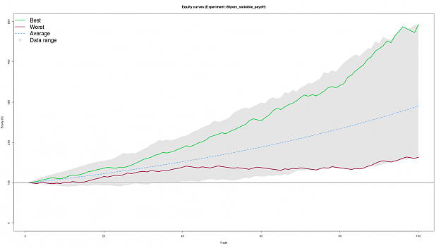
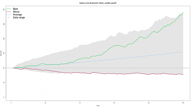
Equity curve plume plot
Attached Image (click to enlarge)
The plume plot shows the range of all the equity curves generated by the simulation (the grey plume in the plots background. The green and dark red lines represent the best and worst curves generated by the simulation. The dashed blue line represents average equity curve for all simulation runs. Positive growth the average line is a good thing.
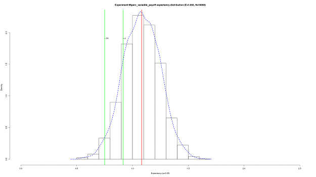
Expectancy histogram
Attached Image (click to enlarge)
Derived from the simulations the histogram shows the variance in the expectancy across all the simulations. The vertical green lines denote 1 and 2 standard deviations less than the mean. The help illustrate that with sufficient pay-off systems with expectancy rates bellow 51% have the potential to be profitable (specifically if 2 standard deviations below the mean is still positive).
The data in this plot can found in the "experiment_name"_expectancies.csv file.
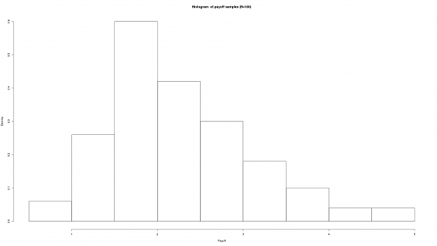
Sample pay-off histogram
Attached Image (click to enlarge)
The generated sample of the potential payoffs used for each of trade in the simulation run. Presented as a diagnostic tool to verify we had the desired distribution in pay-offs.
The following charts demonstrate the for a 45% expectancy a system attain sufficient average reward/pay-off is still profitable (neglecting transnational costs).
The equity curves from the simulation:
Attached Image (click to enlarge)
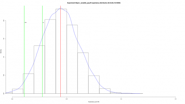
The histogram of the expectancy form 10000 simulations runs of 100 trades each (e.g 1 million simulated trade in total):
Attached Image (click to enlarge)
As you can see 2 (estimated) standard deviations from the (estimated) mean the expectancy is still positive (although not by very much ... especially if transaction costs are thrown into the mix!).
|
Commercial Member
|
Joined Apr 2013
|4,366 Posts
Guys.......The content in this thread is proving to be an excellent resource. Thanks all for sharing. I am going to sit in the background and just absorb the implications of your research. Much obliged all :-)