Historical Daily Returns Distributions

Hi all,

I dug up 15 years of daily prices on 15 currency pairs with the idea of looking at their returns distribution. I wanted to see if there was any chance that a trend-following approach could put us in the direction of a bigger amount of 2-sigma events (daily returns larger then 2 standard deviations). We know that financial time series are not normally distributed but rather have fat tails so I started doing some analysis. I ended up doing a lot more than just this. I'm not claiming this is all 100% accurate or that I have found a holy grail of any kind but I'd like to start some discussion. If anyone is interested and wants to replicate this stuff then perhaps we could falsify some of my results.

I added the historical quotes in attachment. They were extracted from Oanda. If we plot a histogram of the full sample of daily returns we can see that they have a high Kurtosis and definatly not normally distributed:



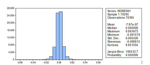
Sample maximum and minimum daily returns are 6.4% and -6.2% respectively. In attachment also the daily return histograms of all pairs individually.

So, I wanted to adopt a "trend-following" approach. I don't think there really is a good measurable way to define a trend. Clearly, I'm simplifying thing here. I construct three exponential moving averages (10,50,200) which corresponds to price being above/below the 10EMA on the MN, W1 and D1 charts together. Turns out that 58% of my observations qualify these criteria which is obviously a lot more than what I hear a lot that markets trend 30% of the time.

Plotting the histograms of daily returns when we are in 'trending up' conditions and when we are in 'trending down' conditions:



mean & median are positive and negative for trending up and trending down respectively. So under the 'trending' conditions, on average, we can expect more positive daily returns when trending up and more negative daily returns when trending down.

kurtosis for both remains high but the skewness I found pretty interesting. My very simple and crude rules seem to tilt the odds a bit in our favor?

Going further, it's obvious that trending up conditions still have large negative moves against us and trending down still have large positive daily returns against us. Let's have a look at the amount of large moves:



When trending up, 3% of daily returns are bigger then 2sigma and 2.6% are smaller then 2sigma. I can't really say much about statistically significant or anything but I found it intruiging. Same goes for trending down: 2.7% are more negative then 2sigma and 2.3% are more positive then 2sigma. Results for 3sigma events are qualitatively similar but clearly, less pronounced.

I went on and tried to see if, by any chance, we could mould this into some sort of system. Every day we check the close of the D1 candle and verify the conditions. If conditions are trending up we would go long and if conditions are trending down we would go short. A trend-following approach should have limited downside and unlimited upside. So I try to implement this: We would go with the direction of the trend every day as long as our conditions hold. This comes down to our 10EMA being our trailing stop. When the D1 closes below this we are no longer considered trending. In addition, we will apply a emergency SL. It's clear that being in an uptrend does not remove negative tail risk. So, every day we place a SL that is X*Sigma below the daily open. I realize that this goes against a very important saying: never make your SL bigger. But the idea is that the 10EMA is the SL and the X*Sigma is an emergency to limit our downside in case there is a large move against us.

So what should X be? We know that in trending conditions about 2.65% is going to be 2*Sigma against us and 0.70% is going to be 3*Sigma against us.

I multiple 'trending down' returns by -1 because we are short here. Add both trending up and trending down together for a total of 40428 observations. This should represent the "true" population because we obviously don't know what the true distribution is...

For X values of -0.005, -0.01 and -0.015 (1*Sigma, 2*Sigma and 3*Sigma) we bootstrap 2500 observations and run this bootstrap 100000 times. This means we randomize our array of 'trending' returns and randomly draw from this array 2500 times. 2500 is probably a bit too small to represent the true distribution of our sample returns but it corresponds to about 1 years worth of trading (40000 obs / 15 pairs) and 100000 tries should converge to the true values? (Not entirely sure about the properties of the estimators here)

We initialize our first row to 5000 which should represent our starting equity and we construct 100000 equity curves based on our bootstrapped returns (=randomly picked from our historical sample with replacement). Like I said, we limit our downside with our emergency stoploss so if the bootstrapped observations is below X*Sigma then we replace it by X*Sigma.

After running, we get a 2500x100000 matrix with equity curves per chosen multiple X. Calculate some basic stats per X:



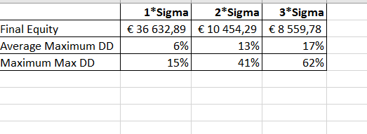
For the 1*Sigma, I drew 200 randomly chosen equity curves:




Let's discuss. Do you think these results are realistic? Can you help me spot some mistakes? Any constructive feedback is welcome!

Best,

You are definitely looking in the right place for a robust strategy. I'd just throw in a couple of comments that might give you some thought based on what I've found in my own similar research:

1. IMHO there is a good objective way to measure a trend - is the price higher or lower than it was X periods ago. I've found that you get best results when the price is both above or below the prices from 3 and 6 months ago.

2. I didn't see why you chose the pairs that you did - I've found that USD pairs have trended far more and more reliably than currency crosses, which tend to mean revert.

The results to me look too good to be true. I'd advise trying it with real data only on lots of pairs, like 25+, or just the USD pairs or USD majors.

Should add there was a regime change around 2008: a 6 month look back worked well before that time but since then 3 months has performed better. Market is choppier since the financial crisis.

You are correct that they look too good to be true. I found some mistakes and the equity curve of this system look more like the one below:



The problem was that I took the system's historical returns as given and those made my system's winrate and by limiting my downside I was essentially boosting my performance by limiting downside more. (stupid mistake). Problem is, I only have daily data so I can not really implement a SL. We never know what happened to price during the day. So limiting my downside should influence my winrate but no way to know how much.

How to define a trend: You seem to be referring to a time series momentum?

The pairs I selected were Majors and Crosses. Interesting statement tho that crosses seem to be more mean reverting. I would think they just combine 2 Majors. So if 2 majors are diverging, their cross would trend even more. And if 2 majors move in the same direction, the cross should indeed be ranging or exhibit mean reversion?

Also interesting: I end up with a negative skew?

Best,

Interesting. Yes, time series momentum is what I meant. I found that I could get good trend following results using only USD pairs, and to a lesser extent Euro crosses, while the results for other crosses on any kind of time series basis has been poor.

This leads to the conclusion that as just about any kind of time series trend following on non-USD and non-Euro crosses leads to bad results, they must be prone to mean-reversion (but I admit I havent thought that through very carefully).

I'm sure if you ran that test with USD only the results would be better.

The discovery about the negative skew is really interesting and I wonder if its not something that we often see on shorter time frames, which is often explained as market makers pushing hard counter-trend to try to shake out trend traders and stop themselves from getting hit too much. Or perhaps it is just the case that when trends eventually end they do so with a bang. Maybe those really negatively skewed days have a probability to signify reversals...?

Thinking about the negative skew.

I don't think the problem lies in my calculations but rather in what we defined and what we are looking at. I plot histograms of daily returns when trending conditions are met.

Pos skew in trend following comes from limiting the downside and having an unlimited upside. This is a system. My histograms doesn't show a system of any kind. It merely shows the expectation of daily returns when conditions of trending are met (very crude definition of a trend). So I think the negative skew comes from the fact that when it ends it often goes against us in a big way and setting us up with a neg skew?


About the trending / mean reversion. I find it a bit difficult to see why they would mean reverting more. I would think that more liquidity => more efficiency (so less trends?). And as crosses are made up off 2 Majors, they should follow this logic. So if EURUSD and GBPUSD are driven by USD strength we can expect EURGBP to be mean reverting to some extent?

Best,

Its an interesting question. I keep finding the data shows trend following based on price data alone for a universe without the USD tends to produce losses. If anyone can contradict that I'd love to see it, and I'm not being sarcastic

Certainly not claiming your statement is incorrect or anything. It'd be interesting to explore further.

Regarding the skewness. If I throw together trending up and trending down returns (trending down*-1 for short positions) and limit my downside to 2*Sigma (~0.01) then we get a trend following returns histogram that sets us up with a pos skew:



So, positive skew in trend following seems to come from trade management i.e. trailing stop of some kind but is not really in the data?

Best,

Hi Guys

Certainly for the past 6 years on the D1 timeframe it appears to be the case. Attached are results of a simple trend following test using >40 instruments (refer to profit matrix) which contains a number of forex pairs. USD pairs rule the roost over this test period. You can see why I devote most of my effort to trading instruments outside the Forex space. In my opinion pairs trading (like Forex) is not great for trend following (but has not always been the case) given you are trading relative strength between different currency pairs and the role Central Banks have had in market intervention practices. The face of trend trading in Forex has changed in recent years with most trend followers needing to stretch further into the longer timeframes to achieve bang for buck. Most of the glorious trends in recent times lie in the commodity space. :-)

PS Note the attached results also include holdings costs so to be fair in any analysis you will see that trends do arise in most of the forex pairs if you disregard this painful feature of trend trading. However USD instruments certainly exhibit great performance over the data set (even including SWAP). Refer to the trade history data if you want to dissect it for further analysis.

PPS Don't get too depressed with the results. 2010 to 2015 has been a difficult period for the medium to long term trend followers. 2010, 2011 and 2012 were real shockers. It has really picked up though at the tail end of 2013 to current.

The decade between 2000 to 2010 was a great period particularly associated with crisis events of 2002 and 2008.

EDIT: I dug this up and thought it might be useful to the discussion. For the purposes of assessing medium term historical trend opportunities for Forex, I have attached a longer range test across Forex pairs (including gold and silver) between 2006 to mid 2015 using another simple trend following strategy.

Wait what?

So if I take a diversified portfolio of instruments traded against some other currency besides the USD it will have a negative expectancy?

If this is what is implied I find this hard to believe. Of course if you are limited to non-USD forex pairs then that isn't really diversity.

I was only talking about Forex.

I can only say that every time I check out any kind of trend trading strategy on Forex over recent years, if you take USD and EUR out of the equation, its a loser.

A quick glance leaves me unconvinced that non-USD pairs should only produce a net loss though I have not done any kind of proper investigation.

It doesn't seem like a project worth pursuing, I don't see the point in trading any non-USD currency pair.