Good evening my fellow traders, I have been a student of the market since 2011 when I joined FF. The entire concept of investing, and obtaining profit through fluctuations in price movement has fascinated me. I have not been fortunate enough to blow accounts as many of you have, I enjoyed relative success in the markets earlier on which fueled my hubris. I erroneously surmised that observing charts, learning patterns, using some sort of money management system and discipline was responsible for my success. I have studied Technical Analysis tools extensively, from MACD,Stochastics, Parabolic SAR, RSI, S/D, S/R, candle stick patterns, you name it.
I have began taking trading seriously lately, not just as an interest and a passion but to dedicate my time in this as a second carrier. I see many here purport to be able to predict price, to "follow" the market, many here will tell me that you have learned the skill to do this successfully. I will respectfully disagree with you, I go as far as to call it Bull shit. In any field of human history where a phenomenon is not well known, not understood, or plainly random... there will be superstition, there will be an array of different methods, some conflicting that will only work due to pure chance. I claim yours is no different.
When studying any such phenomenon, the best tools at our disposal is the scientific method... 1- ask a question, 2- do research, 3- formulate a hypothesis, 4- test your hypothesis, 5- evaluate your results, 6- communicate your findings.
From readying probability theory and statistics I claim that one cannot profit from random data, do you agree with my claim? if you do not let's discuss your ideas here as I am willing to change my mind given the evidence.
If you do not contest my claim then the first question one has to ask is .... is the market random? then null hypothesis should be that it is; unless the evidence points to it not being random.
so how do we test for randomness? let us begin with asking this questions in the statistical sense.... for the data to be random it must follow a random distribution? do you agree? here are two distributions
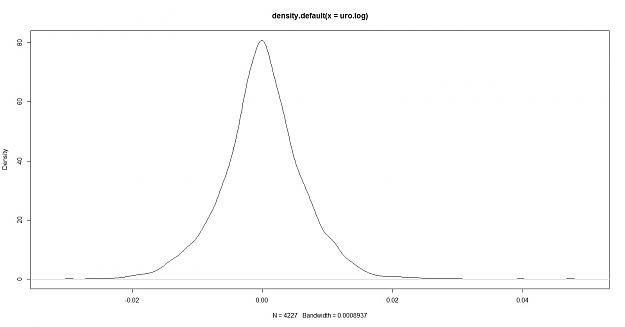
1- fitted to the euro/usd named "DEXUSEU" from the Saint Lous FRED, this data is a total of 4227 euro logarithmic returns
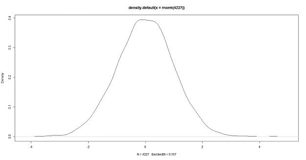
here is the density of a randomly generated data of a sample size of 4227
if we do a QQ plot of euro.log , normally distributed data we can see the fit
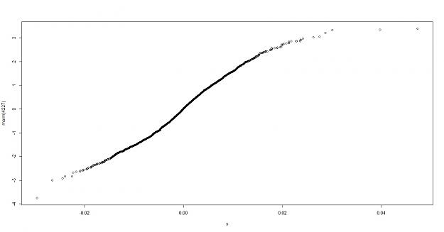
My thoughts: the euro log density appears to have more peakedness and heavier tails, this however only shows that the volatility of the data is different not that it is or isn't predictable. so how do we do a test for randomness?
statistically we would see if there is any serial correlation (auto correlation) meaning: Autocorrelation, also known as serial correlation or cross-autocorrelation,[1] is the cross-correlation of a signal with itself at different points in time (that is what the cross stands for). Informally, it is the similarity between observations as a function of the time lag between them. It is a mathematical tool for finding repeating patterns, such as the presence of a periodic signal obscured by noise, or identifying the missing fundamental frequency in a signal implied by its harmonic frequencies. It is often used in signal processing for analyzing functions or series of values, such as time domain signals.-- wikipedia
here is the auto correlation of a random data
here is also the Partial Auto correlation function:
In time series analysis, the partial autocorrelation function (PACF) gives the partial correlation of a time series with its own lagged values, controlling for the values of the time series at all shorter lags. It contrasts with the autocorrelation function, which does not control for other lags.
This function plays an important role in data analyses aimed at identifying the extent of the lag in an autoregressive model. The use of this function was introduced as part of the Box–Jenkins approach to time series modelling, where by plotting the partial autocorrelative functions one could determine the appropriate lags p in an AR (p) model or in an extended ARIMA (p,d,q) model.
PACF of the Euro
PACF of random data
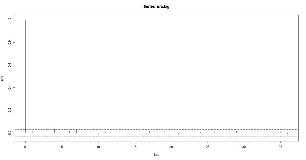
Conclusion: as you can see the Euro does not breach the confidence intervals, the data does not appear to be correlated which supports the null hypothesis of random data. here are the results of the correlation
Autocorrelations of series ‘x’, by lag
0 1 2 3 4 5 6 7 8 9 10 11
1.000 0.012 -0.013 0.000 0.035 -0.035 0.016 0.028 -0.002 -0.003 -0.019 0.006
12 13 14 15 16 17 18 19 20 21 22 23
0.013 0.018 -0.004 -0.012 -0.006 0.013 0.005 0.016 0.008 -0.012 0.011 -0.012
24 25 26 27 28 29 30 31 32 33 34 35
0.008 -0.004 0.007 0.002 0.005 0.017 -0.004 -0.002 -0.003 -0.008 -0.007 0.007
36
-0.011
> acf(rnorm(4227), plot=FALSE)
Autocorrelations of series ‘rnorm(4227)’, by lag
0 1 2 3 4 5 6 7 8 9 10 11
1.000 -0.029 0.034 -0.034 0.010 0.007 0.004 -0.006 -0.002 -0.024 0.009 0.000
12 13 14 15 16 17 18 19 20 21 22 23
-0.015 -0.020 0.006 -0.006 0.013 0.005 -0.003 0.001 0.010 0.002 0.014 -0.002
24 25 26 27 28 29 30 31 32 33 34 35
-0.006 0.011 -0.001 -0.008 -0.013 0.004 0.017 0.004 0.020 -0.012 0.014 0.002
36
-0.007
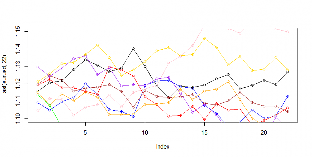
let's look for trend and volatility in the data the first one is euro, the second is a random normally distributed data
I can see a difference in the distribution, the upper red and lower red lines are at sigma one (standard deviations 1 and -1) the red line in the middle is the SMA of 22 = monthly, the yellow lines is the SMA 22*12= 264 which would represent a yearly smoothing, the blue line is to illustrate H=0
Brain sees a difference in the distribution although the monthly smoothing looks similar i can see either real or imagined evidence of trend in the data.
lets look at the Hurst Exponent
> hurstexp(x)
Simple R/S Hurst estimation: 0.5614027
Corrected R over S Hurst exponent: 0.5815521
Empirical Hurst exponent: 0.5223035
Corrected empirical Hurst exponent: 0.5014898
Theoretical Hurst exponent: 0.5211121
> hurstexp(rnorm(4227))
Simple R/S Hurst estimation: 0.5169296
Corrected R over S Hurst exponent: 0.5302739
Empirical Hurst exponent: 0.5114854
Corrected empirical Hurst exponent: 0.4897964
Theoretical Hurst exponent: 0.5211121
the Hurst exponent is another measure of randomness especially Persistence, positive where H>50 H<1 would indicate a trending component while H>0 H<50 would show mean reversion.
The Hurst exponent is used as a measure of long-term memory of time series. It relates to the autocorrelations of the time series, and the rate at which these decrease as the lag between pairs of values increases. Studies involving the Hurst exponent were originally developed in hydrology for the practical matter of determining optimum dam sizing for the Nile river's volatile rain and drought conditions that had been observed over a long period of time.[1][2] The name "Hurst exponent", or "Hurst coefficient", derives from Harold Edwin Hurst (1880–1978), who was the lead researcher in these studies; the use of the standard notation H for the coefficient relates to his name also.
In fractal geometry, the generalized Hurst exponent has been denoted by H or Hq in honor of both Harold Edwin Hurst and Ludwig Otto Hölder (1859–1937) by Benoît Mandelbrot (1924–2010).[3] H is directly related to fractal dimension, D, and is a measure of a data series' "mild" or "wild" randomness.[4]
The Hurst exponent is referred to as the "index of dependence" or "index of long-range dependence". It quantifies the relative tendency of a time series either to regress strongly to the mean or to cluster in a direction.[5] A value H in the range 0.5–1 indicates a time series with long-term positive autocorrelation, meaning both that a high value in the series will probably be followed by another high value and that the values a long time into the future will also tend to be high. A value in the range 0 – 0.5 indicates a time series with long-term switching between high and low values in adjacent pairs, meaning that a single high value will probably be followed by a low value and that the value after that will tend to be high, with this tendency to switch between high and low values lasting a long time into the future. A value of H=0.5 can indicate a completely uncorrelated series, but in fact it is the value applicable to series for which the autocorrelations at small time lags can be positive or negative but where the absolute values of the autocorrelations decay exponentially quickly to zero. This in contrast to the typically power law decay for the 0.5 < H < 1 and 0 < H < 0.5 cases.--wikipedia
finally we can evaluate the Runs Test for randomness
> runs.test(x,plot=TRUE)
Runs Test
data: x
statistic = 2.1203, runs = 2163, n1 = 2080, n2 = 2107, n = 4187, p-value =
0.03398
alternative hypothesis: nonrandomness
> runs.test(rnorm(4227))
Runs Test
data: rnorm(4227)
statistic = 1.3846, runs = 2159, n1 = 2113, n2 = 2113, n = 4226, p-value =
0.1662
alternative hypothesis: nonrandomness
as you can see the P-value on the data x =eur/usd appears be against the null hypothesis of randomness
to conclude my opinion, I claim that with the statistical tools at our disposal it is very difficult to tell the Eurusd data from a Random normally distributed data, therefore T/A alone would be similarly difficult to differentiate from a brownian motion monte carlo simulation and the real market. I claim that you cannot profit from T/A alone, hence the allegations of consistently profiting are highly likely to be false.
I have began taking trading seriously lately, not just as an interest and a passion but to dedicate my time in this as a second carrier. I see many here purport to be able to predict price, to "follow" the market, many here will tell me that you have learned the skill to do this successfully. I will respectfully disagree with you, I go as far as to call it Bull shit. In any field of human history where a phenomenon is not well known, not understood, or plainly random... there will be superstition, there will be an array of different methods, some conflicting that will only work due to pure chance. I claim yours is no different.
When studying any such phenomenon, the best tools at our disposal is the scientific method... 1- ask a question, 2- do research, 3- formulate a hypothesis, 4- test your hypothesis, 5- evaluate your results, 6- communicate your findings.
From readying probability theory and statistics I claim that one cannot profit from random data, do you agree with my claim? if you do not let's discuss your ideas here as I am willing to change my mind given the evidence.
If you do not contest my claim then the first question one has to ask is .... is the market random? then null hypothesis should be that it is; unless the evidence points to it not being random.
so how do we test for randomness? let us begin with asking this questions in the statistical sense.... for the data to be random it must follow a random distribution? do you agree? here are two distributions
1- fitted to the euro/usd named "DEXUSEU" from the Saint Lous FRED, this data is a total of 4227 euro logarithmic returns
Attached Image (click to enlarge)
here is the density of a randomly generated data of a sample size of 4227
Attached Image (click to enlarge)
if we do a QQ plot of euro.log , normally distributed data we can see the fit
Attached Image (click to enlarge)
My thoughts: the euro log density appears to have more peakedness and heavier tails, this however only shows that the volatility of the data is different not that it is or isn't predictable. so how do we do a test for randomness?
statistically we would see if there is any serial correlation (auto correlation) meaning: Autocorrelation, also known as serial correlation or cross-autocorrelation,[1] is the cross-correlation of a signal with itself at different points in time (that is what the cross stands for). Informally, it is the similarity between observations as a function of the time lag between them. It is a mathematical tool for finding repeating patterns, such as the presence of a periodic signal obscured by noise, or identifying the missing fundamental frequency in a signal implied by its harmonic frequencies. It is often used in signal processing for analyzing functions or series of values, such as time domain signals.-- wikipedia
Attached Image (click to enlarge)
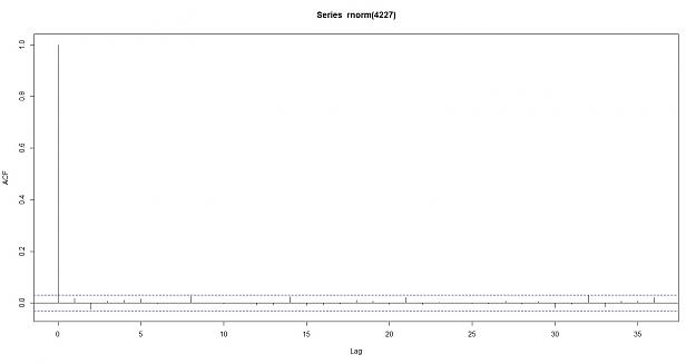
here is the auto correlation of a random data
Attached Image (click to enlarge)
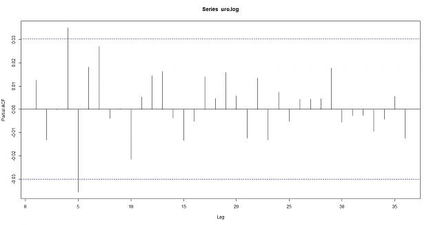
here is also the Partial Auto correlation function:
In time series analysis, the partial autocorrelation function (PACF) gives the partial correlation of a time series with its own lagged values, controlling for the values of the time series at all shorter lags. It contrasts with the autocorrelation function, which does not control for other lags.
This function plays an important role in data analyses aimed at identifying the extent of the lag in an autoregressive model. The use of this function was introduced as part of the Box–Jenkins approach to time series modelling, where by plotting the partial autocorrelative functions one could determine the appropriate lags p in an AR (p) model or in an extended ARIMA (p,d,q) model.
PACF of the Euro
Attached Image (click to enlarge)
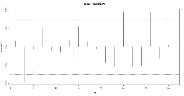
PACF of random data
Attached Image (click to enlarge)
Conclusion: as you can see the Euro does not breach the confidence intervals, the data does not appear to be correlated which supports the null hypothesis of random data. here are the results of the correlation
Autocorrelations of series ‘x’, by lag
0 1 2 3 4 5 6 7 8 9 10 11
1.000 0.012 -0.013 0.000 0.035 -0.035 0.016 0.028 -0.002 -0.003 -0.019 0.006
12 13 14 15 16 17 18 19 20 21 22 23
0.013 0.018 -0.004 -0.012 -0.006 0.013 0.005 0.016 0.008 -0.012 0.011 -0.012
24 25 26 27 28 29 30 31 32 33 34 35
0.008 -0.004 0.007 0.002 0.005 0.017 -0.004 -0.002 -0.003 -0.008 -0.007 0.007
36
-0.011
> acf(rnorm(4227), plot=FALSE)
Autocorrelations of series ‘rnorm(4227)’, by lag
0 1 2 3 4 5 6 7 8 9 10 11
1.000 -0.029 0.034 -0.034 0.010 0.007 0.004 -0.006 -0.002 -0.024 0.009 0.000
12 13 14 15 16 17 18 19 20 21 22 23
-0.015 -0.020 0.006 -0.006 0.013 0.005 -0.003 0.001 0.010 0.002 0.014 -0.002
24 25 26 27 28 29 30 31 32 33 34 35
-0.006 0.011 -0.001 -0.008 -0.013 0.004 0.017 0.004 0.020 -0.012 0.014 0.002
36
-0.007
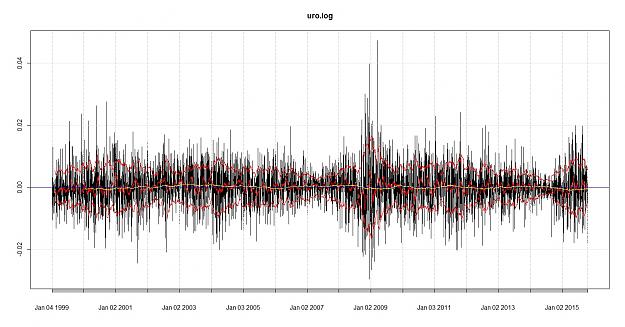
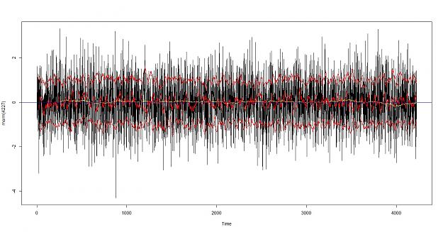
let's look for trend and volatility in the data the first one is euro, the second is a random normally distributed data
Attached Image (click to enlarge)
Attached Image (click to enlarge)
I can see a difference in the distribution, the upper red and lower red lines are at sigma one (standard deviations 1 and -1) the red line in the middle is the SMA of 22 = monthly, the yellow lines is the SMA 22*12= 264 which would represent a yearly smoothing, the blue line is to illustrate H=0
Brain sees a difference in the distribution although the monthly smoothing looks similar i can see either real or imagined evidence of trend in the data.
lets look at the Hurst Exponent
> hurstexp(x)
Simple R/S Hurst estimation: 0.5614027
Corrected R over S Hurst exponent: 0.5815521
Empirical Hurst exponent: 0.5223035
Corrected empirical Hurst exponent: 0.5014898
Theoretical Hurst exponent: 0.5211121
> hurstexp(rnorm(4227))
Simple R/S Hurst estimation: 0.5169296
Corrected R over S Hurst exponent: 0.5302739
Empirical Hurst exponent: 0.5114854
Corrected empirical Hurst exponent: 0.4897964
Theoretical Hurst exponent: 0.5211121
the Hurst exponent is another measure of randomness especially Persistence, positive where H>50 H<1 would indicate a trending component while H>0 H<50 would show mean reversion.
The Hurst exponent is used as a measure of long-term memory of time series. It relates to the autocorrelations of the time series, and the rate at which these decrease as the lag between pairs of values increases. Studies involving the Hurst exponent were originally developed in hydrology for the practical matter of determining optimum dam sizing for the Nile river's volatile rain and drought conditions that had been observed over a long period of time.[1][2] The name "Hurst exponent", or "Hurst coefficient", derives from Harold Edwin Hurst (1880–1978), who was the lead researcher in these studies; the use of the standard notation H for the coefficient relates to his name also.
In fractal geometry, the generalized Hurst exponent has been denoted by H or Hq in honor of both Harold Edwin Hurst and Ludwig Otto Hölder (1859–1937) by Benoît Mandelbrot (1924–2010).[3] H is directly related to fractal dimension, D, and is a measure of a data series' "mild" or "wild" randomness.[4]
The Hurst exponent is referred to as the "index of dependence" or "index of long-range dependence". It quantifies the relative tendency of a time series either to regress strongly to the mean or to cluster in a direction.[5] A value H in the range 0.5–1 indicates a time series with long-term positive autocorrelation, meaning both that a high value in the series will probably be followed by another high value and that the values a long time into the future will also tend to be high. A value in the range 0 – 0.5 indicates a time series with long-term switching between high and low values in adjacent pairs, meaning that a single high value will probably be followed by a low value and that the value after that will tend to be high, with this tendency to switch between high and low values lasting a long time into the future. A value of H=0.5 can indicate a completely uncorrelated series, but in fact it is the value applicable to series for which the autocorrelations at small time lags can be positive or negative but where the absolute values of the autocorrelations decay exponentially quickly to zero. This in contrast to the typically power law decay for the 0.5 < H < 1 and 0 < H < 0.5 cases.--wikipedia
finally we can evaluate the Runs Test for randomness
> runs.test(x,plot=TRUE)
Runs Test
data: x
statistic = 2.1203, runs = 2163, n1 = 2080, n2 = 2107, n = 4187, p-value =
0.03398
alternative hypothesis: nonrandomness
> runs.test(rnorm(4227))
Runs Test
data: rnorm(4227)
statistic = 1.3846, runs = 2159, n1 = 2113, n2 = 2113, n = 4226, p-value =
0.1662
alternative hypothesis: nonrandomness
as you can see the P-value on the data x =eur/usd appears be against the null hypothesis of randomness
to conclude my opinion, I claim that with the statistical tools at our disposal it is very difficult to tell the Eurusd data from a Random normally distributed data, therefore T/A alone would be similarly difficult to differentiate from a brownian motion monte carlo simulation and the real market. I claim that you cannot profit from T/A alone, hence the allegations of consistently profiting are highly likely to be false.
AVT INVENIAM VIAM AVT FACIAM