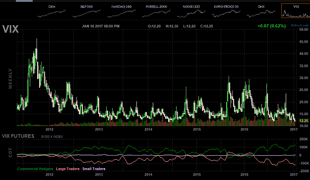
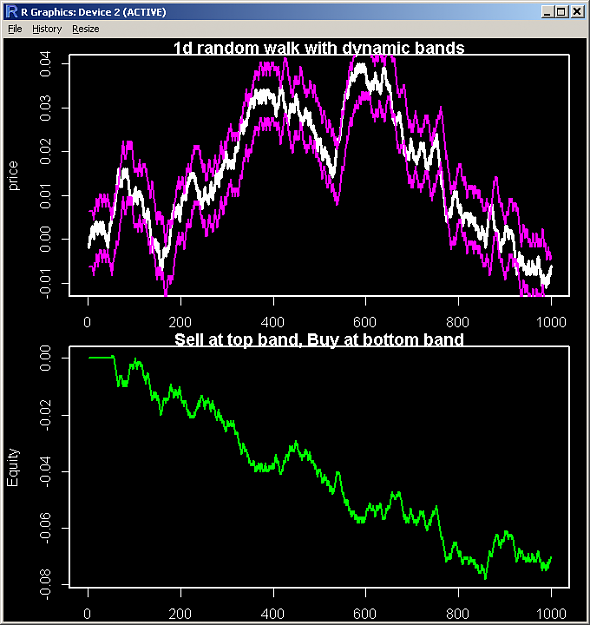
Disliked{quote} The percent of equity (fixed factional) outperforms nearly from the start and continues to increase in its dominance up until about 2000 trades. Then the expectancy based sizing kicks in and just after 2600 trades starts to do better on an absolute basis, and quite dramatically. Any ideas on why this phenomenon might occur in the presence of leverage?Ignored
I have got similar result with the paper.
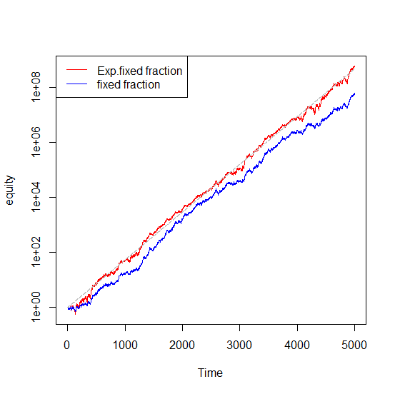
Suppose initial capital is 1, expectancy is 0.2 and fixed fraction is 0.02, which is the same as the paper.
here is my code to create FIGURE 2.
Inserted Code
reward <- 2    #risk is fixed to 1
pwin <- 100 * 1.2/(reward+1)
expectancy <- 0.2
fixed_fraction <- 0.02
w <- numeric(5000*pwin/100) + reward
l <- numeric(5000*(1-pwin/100)) - 1
wl <- c(w,l)
sim <- sample(wl, 5000, replace = FALSE, prob = NULL)
### ff = Fixed Fraction, eff = Expected Fixed Fraction ###
effsize <- 1*(1+expectancy*fixed_fraction)^(1:5000)
ffeq <- numeric(5001) ; ffeq[1] <- 1
effeq <- ffeq
for (i in 2:5001){
ffeq[i] <- ffeq[i-1] + fixed_fraction*ffeq[i-1]*sim[i-1]
effeq[i] <- effeq[i-1] + fixed_fraction*effsize[i-1]*sim[i-1]
}
ffeq <- ffeq[-1]
effeq <- effeq[-1]
ts.plot(effeq,log="y",col=2,ylab="equity")
lines(ffeq,col=4)
lines(cumprod(numeric(5000)+1.004),lty=5,col=8)
legend("topleft", legend = c("Exp.fixed fraction","fixed fraction"), col = c(2,4), lty = 1)
Attached Image
This is how to create FIGURE 4 with other reward:risk ratio (and win rate).
Number of iteration is 1000 to calculate max drawdown and average return.
Inserted Code
library(PerformanceAnalytics)
reward <- c(5, 4, 3, 2, 1.4, 1, 0.6, 0.5)
res <- matrix(0,ncol=length(reward),nrow=11)
res[1,] <- reward
res[3,] <- 0.2
res[4,] <- 0.02
res[6,] <- 1.004
res[7,] <- 1.004^5000

for (k in 1:length(reward)){
pwin <- 100 * 1.2/(reward[k]+1)
geometric_mean <- (1+reward[k]*fixed_fraction)^(pwin/100) * (1-1*fixed_fraction)^(1-(pwin/100))
w <- numeric(5000*pwin/100) + reward[k]
l <- numeric(5000*(100-pwin)/100) - 1
wl <- c(w,l)
me <- numeric(1000) ; me2 <- me  # average ending equity
dd <- numeric(1000) ; dd2 <- dd  # max drawdown
for (j in 1:1000){
 sim <- sample(wl, 5000, replace = FALSE, prob = NULL)
 ffeq <- numeric(5001) ; ffeq[1] <- 1
 effeq <- ffeq
 for (i in 2:5001){
 ffeq[i] <- ffeq[i-1] + fixed_fraction*ffeq[i-1]*sim[i-1]
 effeq[i] <- effeq[i-1] + fixed_fraction*effsize[i-1]*sim[i-1]
 }
 ffeq <- ffeq[-1] ; me[j] <- ffeq[5000]
 effeq <- effeq[-1] ; me2[j] <- effeq[5000]

 a <- xts(ffeq,as.POSIXct("2010-01-01")+c(1:5000)*3600*24)
 dd[j] <- maxDrawdown(diff(a),geometric=F)

 b <- xts(effeq,as.POSIXct("2010-01-01")+c(1:5000)*3600*24)
 dd2[j] <- maxDrawdown(diff(b),geometric=F)
}
res[2,k] <- pwin
res[5,k] <- geometric_mean
res[8,k] <- mean(me)
res[9,k] <- mean(me2)
res[10,k] <- max(dd)
res[11,k] <- max(dd2)
}
rownames(res) <- c("Average win/average loss", "Win%", "Expectancy", "Fixed-fraction",
 "Geometric mean", "Arithmetic mean", "Expected equity", "Fixed-fraction ending equity",
 "Exp. fixed-fraction ending equity", "Max drawdown fixed-fractional", "Max drawdown Exp. fixed-fractional")
And the result(bit messy) is:
Inserted Code
> res
                                                [,1]              [,2]              [,3]              [,4]              [,5]              [,6]              [,7]              [,8]
Average win/average loss                   5.0000000         4.0000000         3.0000000         2.0000000         1.4000000         1.0000000         0.6000000         0.5000000
Win%                                      20.0000000        24.0000000        30.0000000        40.0000000        50.0000000        60.0000000        75.0000000        80.0000000
Expectancy                                 0.2000000         0.2000000         0.2000000         0.2000000         0.2000000         0.2000000         0.2000000         0.2000000
Fixed-fraction                             0.0200000         0.0200000         0.0200000         0.0200000         0.0200000         0.0200000         0.0200000         0.0200000
Geometric mean                             1.0029041         1.0031215         1.0033444         1.0035730         1.0037131         1.0038077         1.0039033         1.0039274
Arithmetic mean                            1.0040000         1.0040000         1.0040000         1.0040000         1.0040000         1.0040000         1.0040000         1.0040000
Expected equity                    466191171.7107646 466191171.7107646 466191171.7107646 466191171.7107646 466191171.7107646 466191171.7107646 466191171.7107646 466191171.7107646
Fixed-fraction ending equity         1981471.9473787   5855907.6056791  17785366.5754087  55578353.2849045 111680121.9162590 178923205.7332271 288082252.9593502 324766199.4659325
Exp. fixed-fraction ending equity  474296490.3162524 460711585.8084800 466129480.0134068 468278620.8666164 469993191.1152020 466338678.3594403 466678983.8887988 474173067.1491528
Max drawdown fixed-fractional              0.9719071         0.9284195         0.9139229         0.7596804         0.6010041         0.4517811         0.3157544         0.2733880
Max drawdown Exp. fixed-fractional        31.6233435         5.7860760         5.9283471         2.9598390         1.4142142         0.9190996         0.4720750         0.3241527
As we can see, Win % decreases with Max drawdown increases.
Within 1000 iterations, only reward:risk=1:1 and smaller reward:risk give max drawdown less than 100% for Exp. fixed-fraction money management.
This is discussed many times and this is why high win rate is preferable.
Yet high winrate system is difficult to create.
##################################
Suppose
win-rate:loss-rate = 50%:50% and
reward is 1% and risk is also 1% of your capital
If you trade 10 times, you get 5 win and 5 loss.
(you can change numbers for profitable/losing system)
The number of path(5win&5loss) is defined as C(n,r) = n!/( r! * (n-r)! )
So the number of path is 10!/( 5! * 5! ) = 252
After the 10 trades, the capital is always the same because A*B=B*A as PipMeUp said.
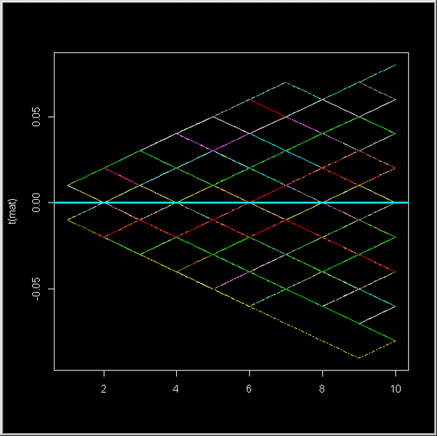
Here is the equity curve and the sample code:
Attached Image
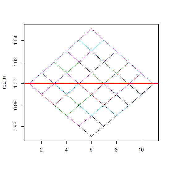
Inserted Code
reward <- 0.01
risk <- 0.01
ntrade <- 10
nloss <- 5
comb <- combn(ntrade, nloss)
mat <- matrix(1+reward,ntrade,ncol(comb))
return <- mat
for (i in 1:ncol(comb)){
mat[comb[,i],i] <- 1 - risk
return[,i] <- cumprod(mat[,i])
}
return <- rbind(1,return)
matplot(return, type="l")
abline(h=1,col=2)
The shape is parallelogram and the final capital is 0.9995001 (less than 1) due to geometric return.
So which path do we prefer?
I prefer something like WLWLWLWLWL and not WWWWWLLLLL because what important is not return itself but risk adjusted return.
We can increase return by increasing postion size (like what Copernicus said in this post).
Therefore, focusing on net profit, profit factor or expected payoff is not good enough.
We must have a look at downside risk like max drawdown, No. of win trade that made higher high, drawdown lengths, etc...
If you are not familiar, search FXEZ's posts or alphaomega's posts with word "drawdown".
They have very good understanding on developing a system and money management.
The problem though is that it is difficult to create a system that reproduces WLWLWL...
We all know markets trend and range. Trend system lose on range market and range system lose on trend market.
The solution is to go into the smaller timeframe and catch the micro trend (momentum) regardless of the market condition.
But retail traders are not very good environment for high frequency trading.
When I read a book Optimize Your Trading Edge by Bo Yoder, he said something like payback/payout cycle.
Can we distinguish payback/payout cycle, and change position size based on the cycle?
I am bit negative and so what I do is exactly the same as alphaomega explained (like stairstep).
Does anyone know the paper/research that talk about improving the performance of particular trading strategy(especially trend trading system-high R:R with Low win%)?
Thank you,
1