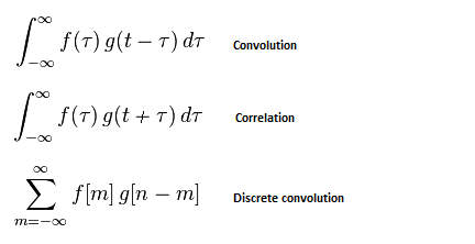
QuoteDislikedWhich gets me to my real question ... any chance you could post the integrals for your convolution?
To me a convolution isn't an infinite integral, its a sigma sign
Also I usually use a compact support: the kernel is zero outside a range [a, b]. So the sigma is from a to b not from minus infinity to plus infinity.
Also when I say convolution it is an abuse of language. It is more precisely a correlation. But if I had written "correlation" you would have thought about something different. The difference between correlation and convolution is the minus sign turning into a plus sign. This is equivalent to mirroring the g(.) function (the kernel) by changing it into G(x)=g(-x). That's why I use the term "convolution".
Attached Image
If you don't know about the convolution operator I agree that the formula is puzzling... Just think about it as a FIR filter or... a moving average!
A SMA(5) is a discrete convolution of the price with the kernel [1,1,1,1,1]
A LWMA(5) is a discrete convolution of the price with the kernel [5,4,3,2,1]. Notice that the kernel is "reversed". The LWMA(5) is a correlation with the kernel [1,2,3,4,5].
The delta function is the neutral element of the convolution that is if you convolve delta with any kernel you get this kernel. This is the impulse response of a FIR filter for the signal processing people.
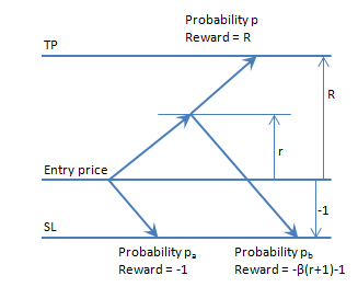
Say you have 60% chance losing 1 and 40% chance winning 2. You can represent this as a correlation kernel [0, 0.6, 0, 0, 0.4]. The middle value is the current equity.
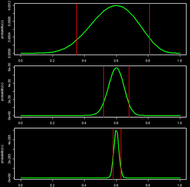
Let's say your starting equity is 100. You can reprensent this as a probability distribution which is 1 at 100 and 0 everywhere else.
In discrete space it looks like [0, 0, 0, ..., 0, 1, 0, ..., 0, 0] with the 1 at index 100.
Inserted Code
# You need the package signal to get conv()

# Starting equity
eq <- c(rep(0,100), 1, rep(0,100));
plot(eq, t='h');

# PDF of the game
kernel <- c(0,0.6,0,0,0.4);

# New possible equities after step 1
eq <- conv(eq, kernel);
plot(eq, t='h');

# New possible equities after step 2
eq <- conv(eq, kernel); plot(eq, t='h');

# Repeat as many times as you want...
Attached Image (click to enlarge)
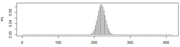
On the topic of doing this in R... I was unable to build the equivalent of a for-loop with the *apply functions family. The variables scoping seems like the inner function sees a new copy of the variables... The eq vector is reset to the starting value at each iteration.
I wanted to store each histogram as a column vector of a matrix. Then drawing the matrix (with image() or plot2d()?) one should get something looking like your MC graphs but including ALL the possible futures as a color height map representing the probability of the equity.
No greed. No fear. Just maths.