Let's see how the sampling influences the real life data. I took the data from E/U versus U/CHF over 2012. The reason for this choice is the SNB peg on EUR/CHF. When a central bank maintains EUR/CHF at almost exactly 1.2000, E/U and U/CHF can only be perfectly correlated since EUR/CHF = EUR/USD / USD/CHF at any time. This very special situation gives me a reference for 2 perfectly correlated pairs. Thank you SBN!
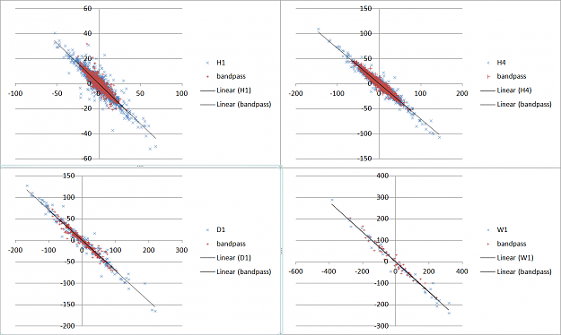
In regard to the previous post I removed the trend and the noise with a IIR Butterworth band pass filter (band 0.2 - 0.6 normalized frequency if you want to know; code from http://www-users.cs.york.ac.uk/~fisher/mkfilter/). The results are in the picture. Remarkably the regression is almost exactly the same with and without the filtering for the 4 TF I tested. After filtering the data is more compact (they are the red dots).
I mesure the alignment of the cloud on the trendline with the formula 1-squareRoot(e2/e1). Where e1 and e2 are respectively the first and the second eigenvalues of the co-variance matrix. I also mesure the regression coefficient (the slope of the regression line). For the dataset I expect 1 for the dispersion, i.e. a perfect cointegration, as any move of one pair must be counter-balanced by the other one to keep EUR/CHF constant. The result are
W1 - regression 0.70 - cointegration 0.90
D1 - regression 0.71 - cointegration 0.89
H4 - regression 0.70 - cointegration 0.84
H1 - regression 0.64 - cointegration 0.83
W1 which has got the smallest set of samples is surprisingly the nearest of the expected cointegration index with 0.9. Daily gives the same result. H4 and H1 don't perform very well.
The regression is the same for W1, D1 and H4. This consensus seems to lead to the thinking 0.7 is somewhat the correct value. H1 is completely off.
D1 and W1 are the two best TF to mesure my risk index. Daily contains more samples and will react more quickly so now on I'll use D1.
Attached Image (click to enlarge)
No greed. No fear. Just maths.
